Linear regression with Python
Ejemplo de cómo ajustar un modelo de regresión lineal con Python usando sklearn y graficarlo con matplotlib.
#libraries used
import numpy as np
from sklearn.linear_model import LinearRegression
import matplotlib.pyplot as plt

#Data
x = np.array([20, 40, 60, 80, 100, 120])
y = np.array([220, 200, 180, 170, 150, 135])

#Creating the linear_regression object
linear_regression = LinearRegression()
linear_regression.fit(x.reshape(-1, 1), y)

#The linear model: y = m*x + b
#=========================================

#Intercept with y-axis
b = linear_regression.intercept_

#Slope
m = linear_regression.coef_

#Showing the results
print(f"The intercept is: {b:.3f}")
print(f"The slope is: {m[0]:.3f}")

#Plotting the data x and y, and the linear equation
plt.scatter(x, y, color = "blue")
plt.plot(x, m*x + b, color = "red")
plt.xlabel("x")
plt.ylabel("y")
plt.title("Linear Regression")
plt.grid()
plt.show()
Al ejecutarlo obtenemos el siguiente gráfico:
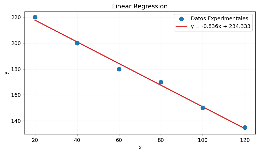
El modelo lineal \(y = m \cdot x + b\) se ajusta a los puntos minimizando la suma de cuadrados de los residuos:
\[\min_{m,\,b} \sum_{i=1}^{n} \left(y_i - (m\,x_i + b)\right)^2\]
Derivando respecto a \(m\) y \(b\) e igualando a cero se obtienen las ecuaciones normales:
\[\frac{\partial S}{\partial m} = -2 \sum_{i=1}^{n} x_i \left(y_i - m\,x_i - b\right) = 0\]
\[\frac{\partial S}{\partial b} = -2 \sum_{i=1}^{n} \left(y_i - m\,x_i - b\right) = 0\]
Despejando, las estimaciones de mínimos cuadrados quedan:
\[m = \frac{\sum_{i=1}^{n} (x_i - \bar{x})(y_i - \bar{y})}{\sum_{i=1}^{n} (x_i - \bar{x})^2} \qquad b = \bar{y} - m\,\bar{x}\]
donde \(\bar{x}\) y \(\bar{y}\) son los promedios de \(x\) e \(y\) respectivamente.